Have you ever wondered how those lines on a badminton court get detected in videos? This article is all about that! We will take a peek into the cool technology behind spotting those lines using cameras. We will keep it simple, exploring how computers ‘see’ and learn to recognize the lines. Think of it as a behind-the-scenes tour of the tech that helps iSportz understand and analyze sports better. So, get ready to dive into the world of video analysis and discover how these nifty innovations make a big difference in the game.
This technology is not just about making the game more exciting to watch. It is also a game-changer for players and coaches. By accurately identifying court lines, coaches can analyze player positioning, strategy effectiveness, and even detect faults. Players can review their performance with detailed insights, improving their skills with each game. So, whether you are a fan, a player, or simply curious about the wonders of sports tech, buckle up for an enlightening journey into the world of line detection technology.
At iSpotz, we have crafted a meticulous process for court line detection, laying the foundation for advanced video analytics to enhance player performance. Let’s walk through our step-by-step approach:
- Convert Image to Grayscale: When we convert an image to grayscale, we essentially strip away its colors, leaving behind only shades of gray. This process simplifies the image, making it easier to analyze because we are now solely focused on variations in brightness or intensity of light across the image. By removing color information, we streamline the subsequent analysis steps, as we no longer have to deal with the complexities that come with different color channels. Instead, we can concentrate on detecting edges, lines, and other features based solely on the varying levels of brightness in the image. This simplification helps in achieving more accurate and efficient image processing and analysis.
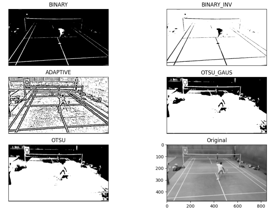
- Image Binarization: Binarization is a handy tool in image processing that helps simplify images. When we binarize an image, we convert it into a binary form, which means it only contains two colors: black and white. In this process, black usually represents the background, while white represents the object or the part we are interested in. This step is essential in many computer vision and image analysis tasks. To binarize an image, we first pick a threshold value. Then, we make all pixel values below that threshold black and those above it white. We analyzed below techniques for binarization:
a. Global Thresholding:
- In global thresholding, we used a single fixed value as a threshold for all pixels (we considered 190 on analyzing histogram).
- We compare each pixel’s intensity in the image with this threshold value.
- If the intensity is greater than the threshold, we set the pixel value to 255 (white); otherwise, we set it to 0 (black).
- This method assumes that the image has a clear separation between background and foreground, making it suitable for images with consistent lighting.
b. Adaptive Thresholding:
- Unlike global thresholding, adaptive thresholding we calculated different threshold values for different image regions.
- This method helps overcome issues with variable lighting and shading.
- Two common adaptive thresholding techniques in OpenCV are Adaptive Mean Thresholding and Otsu Thresholding.
c. Otsu Thresholding:
- Otsu’s method automatically selects the optimal threshold value by assuming a bimodal distribution of pixel intensities in the image.
- It finds the threshold value that minimizes the weighted variance between background and foreground pixels, effectively separating them.
- By iteratively testing different threshold values, Otsu’s method identifies the threshold that maximizes the inter-class variance or minimizes the intra-class variance.
- This technique is particularly useful when the distribution of pixel intensities in the image is not known beforehand.
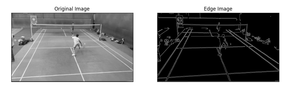
3. Canny Edge Detection: Canny Edge Detection is a widely used algorithm for detecting edges in images, developed by John F. Canny. It operates in multiple stages, each crucial for accurate edge detection.
a. Noise Reduction:
- To begin, the algorithm addresses noise in the image by applying a 5×5 Gaussian filter, which smoothes out irregularities.
b. Finding Intensity Gradient:
- Next, the smoothed image undergoes filtering with a Sobel kernel in horizontal and vertical directions to compute the gradient (rate of change) of intensity.
- The gradient magnitude and direction are calculated for each pixel using the formula

Gx represents the gradient in the horizontal direction.
Gy represents the gradient in the vertical direction.
θ (theta) represents the direction of the gradient.
- The gradient direction is rounded to one of four angles representing vertical, horizontal, and two diagonal directions.
c. Non-maximum Suppression:
- This stage identifies true edges by removing redundant pixels.
- A pixel is considered an edge only if it’s a local maximum in the direction of the gradient.
- Any pixel that does not qualify as a local maximum is suppressed (set to zero), resulting in a binary image with thin edges.
d. Hysteresis Thresholding:
- Finally, this stage determines which detected edges are genuine.
- It employs two threshold values, minVal and maxVal.
- Pixels with intensity gradients above maxVal are considered sure-edges, while those below minVal are discarded as non-edges.
- Pixels between minVal and maxVal are classified based on connectivity to sure-edge pixels.
- Edges connected to sure-edge pixels are retained, while disconnected edges and noise are eliminated.
- This process effectively filters out small pixel noises and ensures that only strong edges remain in the final image.
In essence, Canny Edge Detection produces a binary image highlighting the strong edges, providing a clear representation of the image’s features.
4. Hough Transformation: The Hough transform is a powerful method used to identify specific shapes within an image. It’s particularly effective for detecting regular curves like lines, circles, and ellipses. While the classical Hough transform focuses on well-defined shapes with parametric representations, a generalized version can handle more complex features lacking simple descriptions. The Hough technique is adept at generating a comprehensive description of features across an image, even when dealing with noise or incomplete boundary data. It operates by assigning significance to each local measurement, such as a coordinate point, in contributing to a global solution. For instance, in line detection, every point in the image indicates its relevance to a potential line present in the scene. This approach enables the Hough transform to robustly identify features regardless of gaps in boundary information or image noise.
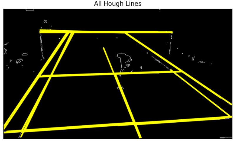
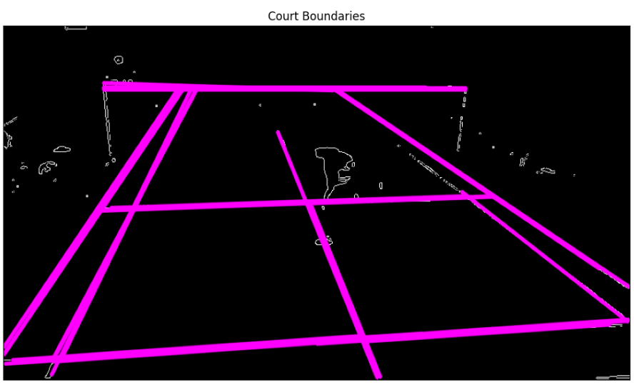
5. Draw Detected Lines
For visualization, you can draw the detected lines back onto the image. This step helps you see which lines the Hough Transform found.
6. Find Intersection of boundary Hough Lines:
Finding the determinant of two line segments using the below formula will return the intersection point of those two lines.
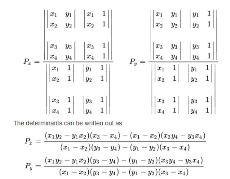
So now if we loop through all our lines, we will have intersection points from all our horizontal and vertical lines.
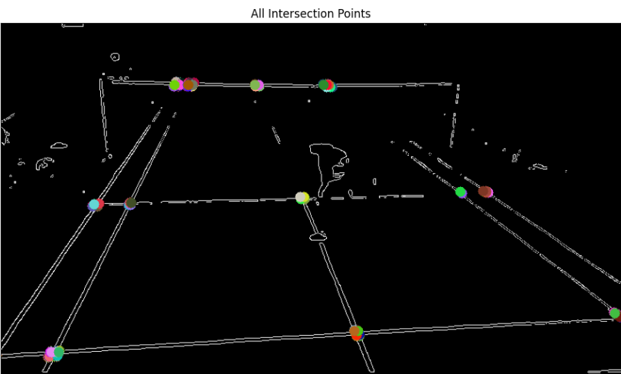
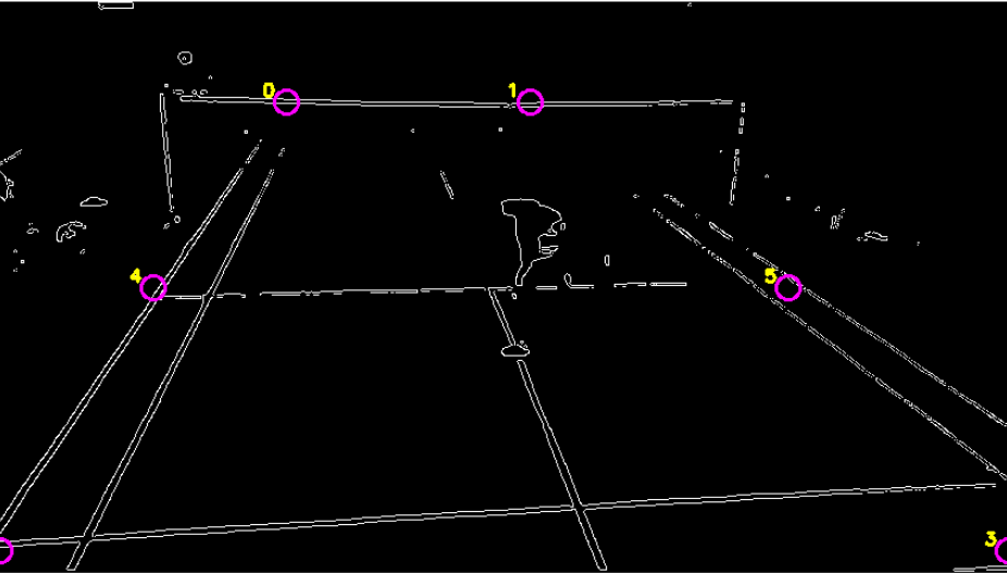
When we loop through all our detected lines to find intersection points between horizontal and vertical lines, we end up with numerous intersection points. This happens because our line detection algorithm identifies multiple lines that are very close to each other, resulting in several intersection points clustered around the same corner of a box.
Conclusion:
In our journey through the technology behind video-based court line detection in badminton, we have explored the fascinating intersection of computer vision and sports analytics. Using powerful tools like the Hough Transform, we can detect and analyze lines within an image, even when dealing with challenges like varying angles and lighting conditions.
By following a systematic approach—starting with preprocessing the image, detecting edges, applying the Hough Transform, and refining our results through clustering and averaging techniques—we have seen how it is possible to accurately identify the boundary lines on a badminton court. This technology not only enhances the accuracy of line calls in professional matches but also opens up new possibilities for training and analysis in the sport.
From the initial edge detection to the final visualization of line intersections, each step builds upon the previous one, demonstrating the power and precision of modern computer vision techniques. As we continue to innovate and refine these methods, the potential applications in sports and beyond are truly exciting.
Thank you for joining us on this exploration of court line detection. Whether you are a sports enthusiast, a tech geek, or both, we hope this deep dive has given you a new appreciation for the sophisticated technology that powers the sports we love.